Steel Shear Link

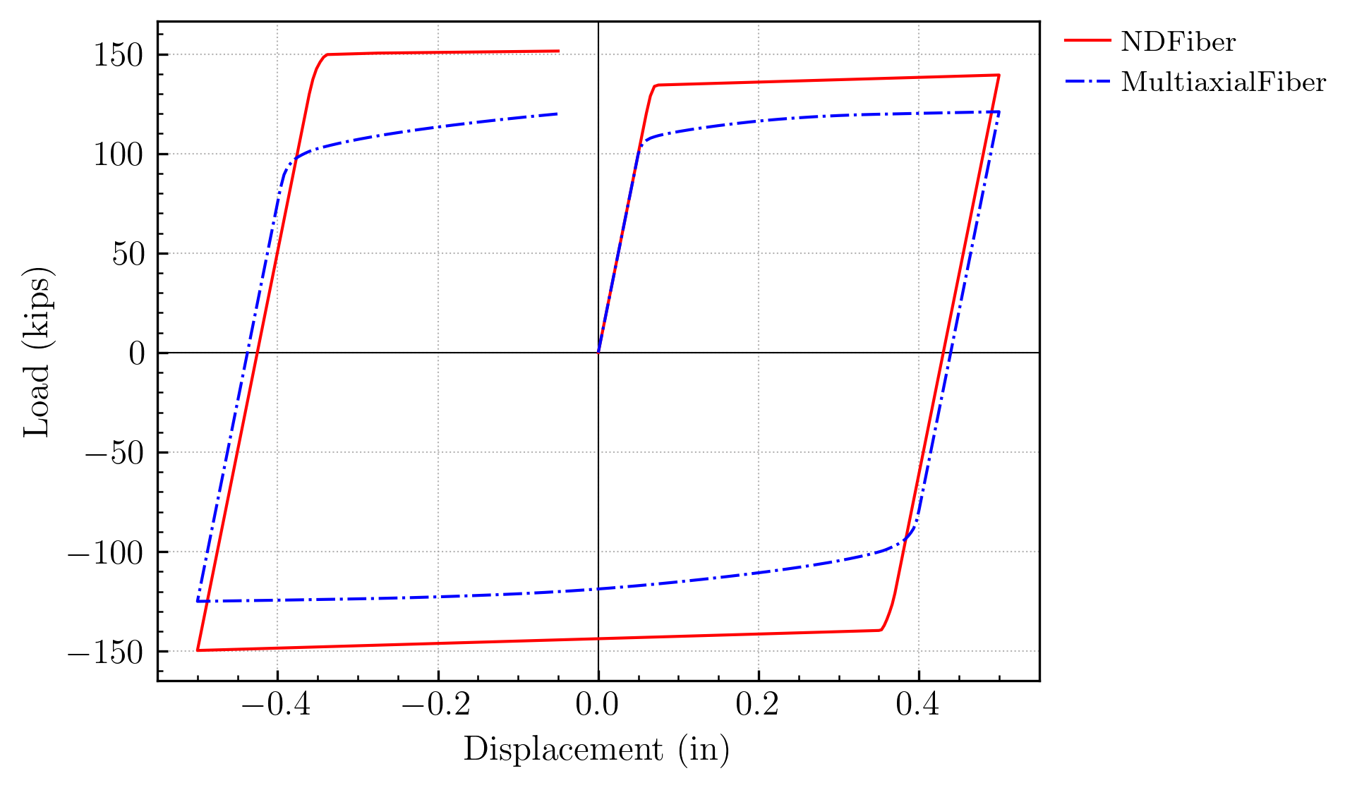
Download notebook

This example compares the shear response of the MultiaxialFiber section with the NDFiber section of OpenSees.

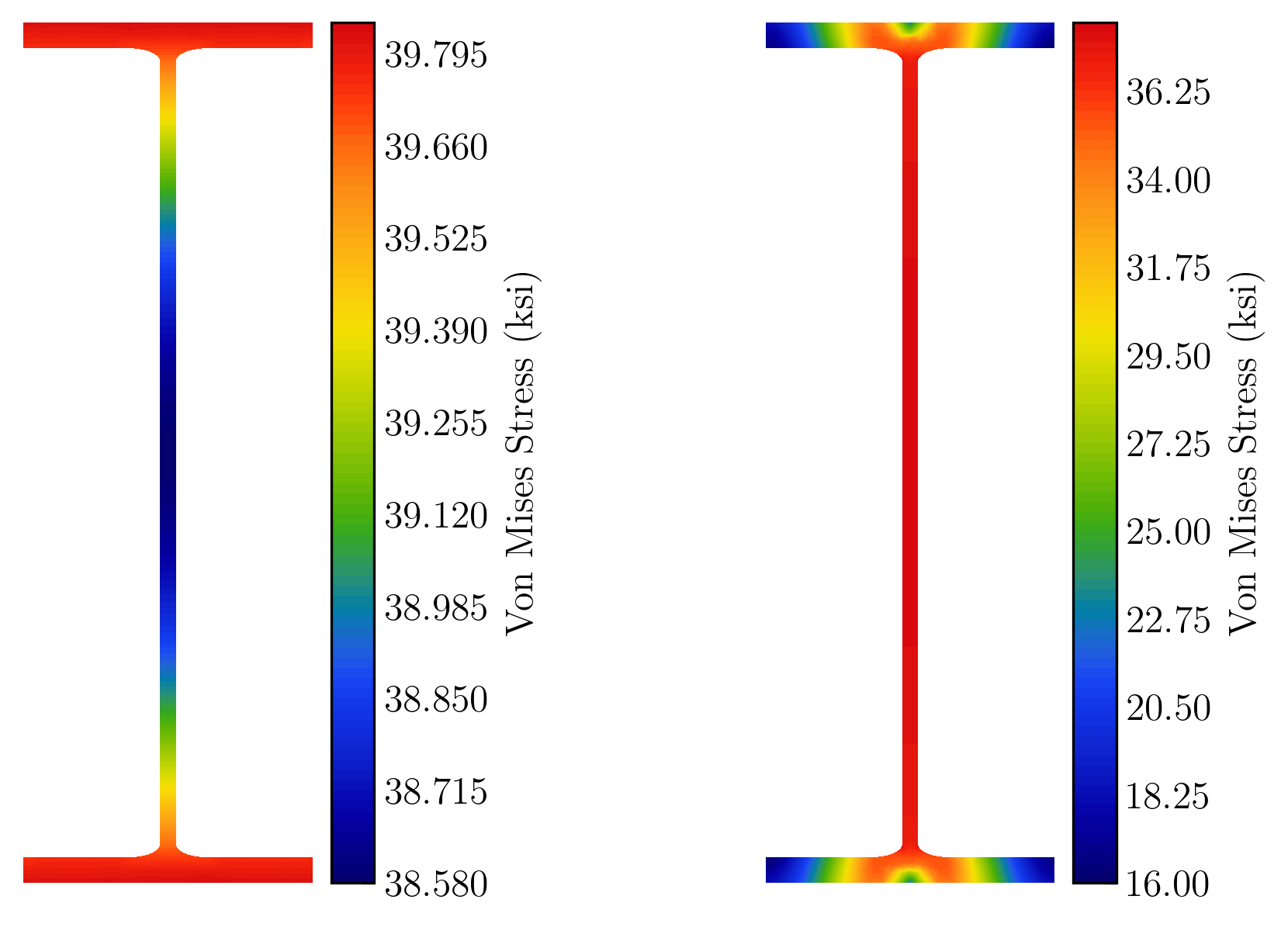
It is demonstrated that NDFiber produces a poorer representation of the link’s shear capacity.

Modeling

import xara
import veux

import xara.units.iks as units
from xara.helpers import find_node

Material

Begin by defining a xara.MultiaxialMaterial using the PlasticJ2 formulation.

Fy = 35.0*units.ksi
E  = 30e3*units.ksi
G  = 12e3*units.ksi

Aspect = 1.5

material = xara.MultiaxialMaterial(
    type="PlasticJ2",
    E =  E,
    G =  G,
    Fy = Fy,
    Hiso = 0.002*E,
    Hkin = 0.002*E
)

Section

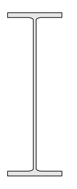
Next, a shape object is created using the from_aisc function.

This will be used to generate fibers with appropriate shear properties, like the shear correction factor \(\kappa\) used by NDFiber and the warping shapes \(\varphi\) used by MultiaxialFiber.

from xsection.library import from_aisc

shape = from_aisc("W18x40",
                units=units,
                mesh_scale=1,
                material=material,
                fillet=True,
                mesh_type="T3",
                mesher="gmsh")

veux.draw_shape(shape)

Finally, the xara.FrameSection objects are created with the two formulations of interest.

sections = [
    xara.FrameSection("NDFiber", shape),
    xara.FrameSection("MultiaxialFiber", shape)
]

veux.draw_shape(sections[1])

Model

L = shape.d*Aspect

def create_model(length, section, material):
    model = xara.Model(ndm=3, ndf=6)
    
    model.node(1, (     0, 0, 0))
    model.node(2, (length, 0, 0))

    model.fix(1, (1,1,1,  1,1,1))
    model.fix(2, (1,1,0,  0,1,1))

    model.material(material)
    model.section(section)

    model.geomTransf("Linear",  1, (0, 0, 1))
    model.element("ForceFrame", 1, (1,2), 
                  section=section, 
                  shear=1, 
                  transform=1)

    return model

Loading

The following create_loads function sets up the loading:

• A xara.TimeSeries is created to define the cyclic loading history

• A xara.NodalValue object is created to impose the value of the displacements of the node with tag ctrl_node in DOF number 3

• A xara.StaticPattern is created assigning the TimeSeries to the NodalValue constraint

def create_loads(model, ctrl_node):

    a = 0.1

    series = xara.TimeSeries(values=[0,  0.05,   0.5, -0.5, -0.05],
                             time=  [0,   a,      1,    4,    5 ])

    # Create the control load
    ctrl = xara.NodalValue(model, node=ctrl_node, dof=3, value=1.0)

    pattern = xara.StaticPattern(ctrl, series=series)

    model.pattern(pattern)

Analysis

The analyze function takes the xara.Model and creates an appropriate analysis object:

• xara.StaticAnalysis oversees a static analysis

def analyze(model, ctrl_node, plots=()):

    # Loading
    step = 100
    analysis = xara.StaticAnalysis(model,
                                   integrator=xara.LoadFactorControl("Proportional", 1/step),
                                   system="BandGeneral",
                                   constraints="Transformation", 
                                   test=("Energy", 1e-18, 20, 0))

    for _ in range(step*5):
        if model.state.time >= 5.0:
            break

        if analysis.analyze(1) != 0:
            print(f"Failed at time = {model.state.time}")
            return

        for plot in plots:
            plot.update(model)

import matplotlib.pyplot as plt
from post import PlotResponse
from xara.post import FiberStress

##
plot_1 = PlotResponse()


_,plot_stress = plt.subplots(1,2)
plot_stress[0].figure.subplots_adjust(wspace=0.8)

##

for i,section in enumerate(sections):


    print(f"Running {section.type}")

    model = create_model(L, section, material)

    ctrl_node = find_node(model, x=L)

    create_loads(model, ctrl_node)

    plot_1.reset(model,
                node=ctrl_node, 
                dof=3,
                label=section.type
    )


    analyze(model, ctrl_node, plots=[plot_1])

    plot_1.draw()

    # Plot stress distribution at the end of the analysis
    artist = veux.ShapeArtist(shape, ax=plot_stress[i])
    artist.draw_surfaces(
        field=FiberStress(model, shape, section=1, stress="svm", element=1),
        cbar_label="Von Mises Stress (ksi)",
    )


plot_1.finish()

Running NDFiber
Running MultiaxialFiber

References

• C. M. Perez, “Nonlinear modeling of frame members for rapid infrastructure assessment,” Ph.D., University of California, Berkeley, Berkeley, CA, 2026. Available at: https://escholarship.org/uc/item/3zn367p3