Finite Rotations#
Download notebookA cantilever beam is investigated under the action of a point moment \(\boldsymbol{M}\) at its free end \(\xi=L\).
The following parameters are used:
Modeling#
Section properties are defined using the Elastic section as follows:
import xara

EI = 1e2
length = 10.0

section = xara.FrameSection("Elastic",
              E=1e4,
              G=1e4,
              A=1,
              Iy=1e-2,
              Iz=1e-2,
              J=1e-2)
The simulation uses a uniform meshes of ne elements. To reproduce the results of Perez and Filippou (2024), use the Spherical transform with the CosseratFrame element.
def create_prism(length:    float,
                 element:   str = "CosseratFrame",
                 transform: str = "Spherical",
                 divisions: int = 5
                 ):

    # Number of elements discretizing the member
    ne = divisions


    model = xara.Model(ndm=3, ndf=6)

    # Total number of nodes
    nn = ne + 1

    # Create nodes
    for i in range(1, nn+1):
        x = (i-1)/float(ne)*length

        model.node(i, (x, 0.0, 0.0))

    # Define boundary conditions
    model.fix(1, (1,1,1, 1,1,1))

    # Define cross-section
    model.section(section)

    # Define geometric transformation
    model.geomTransf(transform, 1, (0, 0, 1))

    # Define elements
    for i in range(1, ne+1):
        model.element(element, i, (i, i+1),
                    section=section,
                    transform=1)

    return model
Analysis#
The function analyze is defined, which runs an analysis under a moment given by
import numpy as np

def analyze_moment(lamda, ne=5, element="CosseratFrame", transform="Spherical"):

    model = create_prism(
        length    = length,
        element   = element,
        transform = transform,
        divisions = ne
    )

    M = 2*np.pi*(EI/length)*lamda

    model.pattern("Plain", 1, "Linear", load={
        ne+1: [0, 0, 0] + [0, 0,  M]}
    )


    analysis = xara.StaticAnalysis(model,
                                   test=("EnergyIncr", 1e-14, 10, 0),
                                   system="BandGeneral"
                                   )
    analysis.analyze(1)

    return model
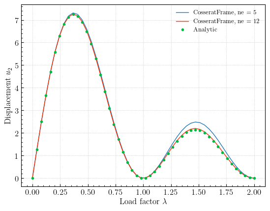
The analysis is performed at \(50\) linearly spaced values of \(\lambda\) between \(0\) and \(2\), where the beam rolls up onto itself twice. For each value of \(\lambda\) a new analysis is performed, so that the full load is solved with only 1 step, and an anamation frame is drawn. Because this problem involves finite rotations, the nodeRotation method is used (as opposed to nodeDisp) to render the nodal rotations.
load = np.linspace(0, 2.0, 50)
#
#

import veux
from veux.motion import Motion

model = analyze_moment(2.0)

artist = veux.create_artist(model,
                            vertical=2,
                            model_config=dict(
                                extrude_outline="square",
                                extrude_scale=0.01
                            ))

motion = Motion(artist)

for m in load:
    model = analyze_moment(m)
    motion.draw_sections(rotation=model.nodeRotation,
                         position=model.nodeDisp)
    motion.advance()

motion.add_to(artist.canvas)
artist
Results#
The solution requires only two iterations for each formulation.
The analytic solution of the governing boundary value problem is given by:
where \(\vartheta\) parameterizes the rotation \(\boldsymbol{\Lambda}(\xi) = \operatorname{Exp} \vartheta(\xi) \, \mathbf{E}_3\).
import matplotlib.pyplot as plt

fig,ax = plt.subplots()

# plot the numerical solutions for 5 and 12 elements
for ne in 5, 12:
    uy = [analyze_moment(m, ne=ne).nodeDisp(ne+1,2) for m in load]
    ax.plot(load, uy, label=f"CosseratFrame, {ne = }")


# plot the analytic solution
def solution(lamda):
    M = 2*np.pi*(EI/length)*lamda
    theta = length * M / EI
    return -(EI/M)*(np.cos(theta) - 1.0)

ax.plot(load, [0]+[solution(m) for m in load[1:]], ".", label="Analytic")


ax.set_xlabel(r"Load factor $\lambda$")
ax.set_ylabel(r"Displacement $u_2$")
ax.grid(True)
ax.legend();
References#
C. M. Perez and F. C. Filippou, “On nonlinear geometric transformations of finite elements,” Numerical Meth Engineering, vol. 125, no. 17, Sep. 2024, doi: 10.1002/nme.7506.
NAFEMS Finite Element Methods & Standards, Abbassian, F., Dawswell, D. J., and Knowles, N. C., Selected Benchmarks for Non-Linear Behavior of 3D-Beams. Glasgow: NAFEMS, Publication NNB, Rev. 1, Oct. 1989. Test NL5.