Plasticity

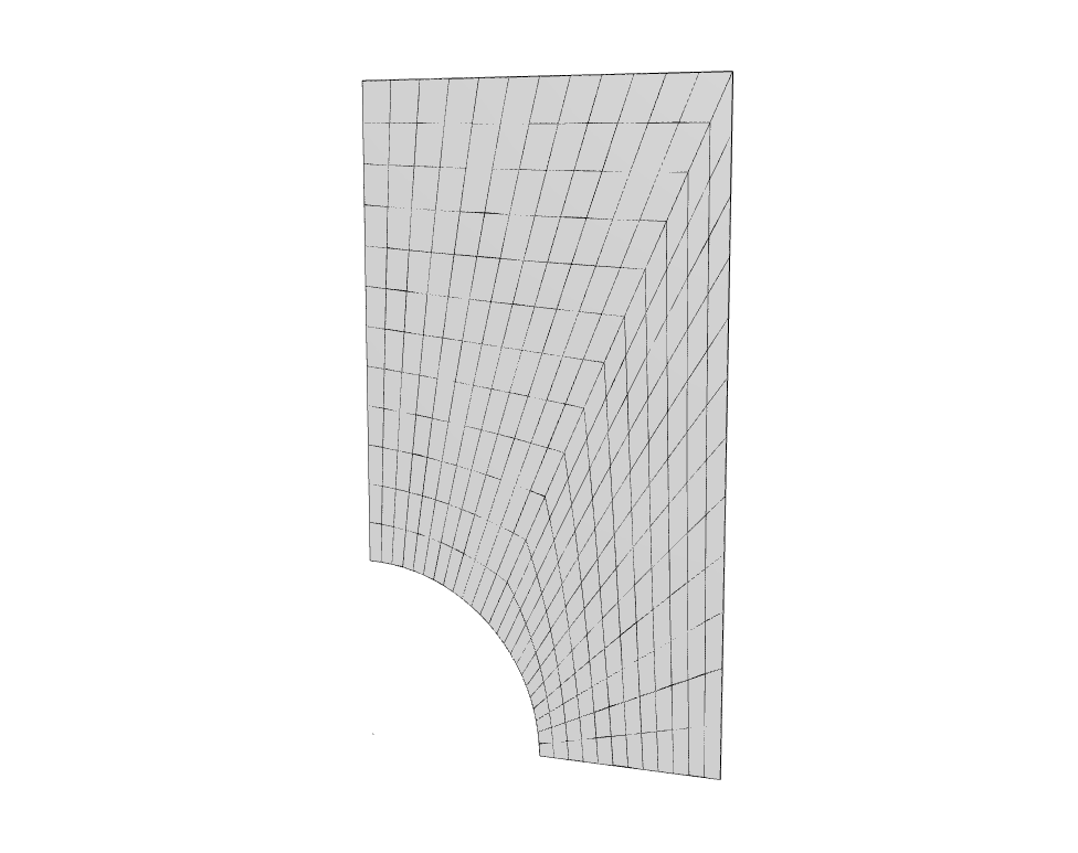
Download notebook

An inelastic steel plate is modeled. The geometry is as shown below.

Modeling

Dimensions

from xara.units import create_units

units = create_units(system="iks")
meter = units.meter
MPa   = units.MPa

radius =  5*meter
width  = 10*meter
length = 18*meter
thickness = 1.0

Create the xara.MultiaxialMaterial using the PlasticJ2 formulation:

import xara 
material = xara.MultiaxialMaterial(
    type="PlasticJ2",
    E=70*MPa,
    nu=0.2,
    Fy=0.243*MPa,
    Hiso=0.0*MPa,
    Hkin=0.0*MPa,
    tol=1e-12
)

Next create a xara.PlaneSection to model the plane strain condition:

section = xara.PlaneSection("PlaneStrain", material, thickness)

Now the xara.Model is created and populated.

import numpy as np

model = xara.Model(ndm=2, ndf=2)

# Add the material and section to the model
model.material(material)

model.section(section)

model.surface(
    (12,12),
    element="quad",
    args={"section": section},
    points={
        1: (0, radius),
        5: (radius*np.cos(np.pi*3/8), radius*np.sin(np.pi*3/8)),
        2: (radius*np.cos(np.pi/4), radius*np.sin(np.pi/4)),
        3: (width, length),
        4: (0, length)
    }
)

model.surface((12,12),
    element="quad",
    args={"section": section},
    points={
        1: (radius*np.cos(np.pi/4), radius*np.sin(np.pi/4)),
        5: (radius*np.cos(np.pi/8), radius*np.sin(np.pi/8)),
        2: (radius, 0),
        3: (width, 0),
        4: (width, length)
    }
);

Use the veux library to render the model:

import veux
veux.render(model)

Boundary

Next, fix all degrees of freedom at the base. For this we’ll use the find_nodes helper function, which allows us to iterate over all node tags in the xara.Model with specified x or y coordinates:

from xara.helpers import find_nodes

for node in find_nodes(model, y=0):
    model.fix(node, (0, 1))

for node in find_nodes(model, x=0):
    model.fix(node, (1, 0))

Loading

The loading for this problem involves imposing a vertical displacement at the nodes found along the top edge of the mesh.

For this purpose, we populate a xara.StaticPattern with xara.NodalValue objects created for each Node tag that is returned from find_nodes(model, y=length)

pattern = xara.StaticPattern([
    xara.NodalValue(model, node, 2, 1.0) 
    for node in find_nodes(model, y=length)
])

Once the xara.StaticPattern is created it must be added to the xara.Model:

model.pattern(pattern)

1

Analysis

step = 1 #0.1

analysis = xara.StaticAnalysis(model,
                               system="Umfpack",
                               algorithm=("NewtonLineSearch", 0.6),
                               constraints="Transformation",
                               test=("Energy", 1e-16, 20, 0),
                               integrator=("LoadControl", step))

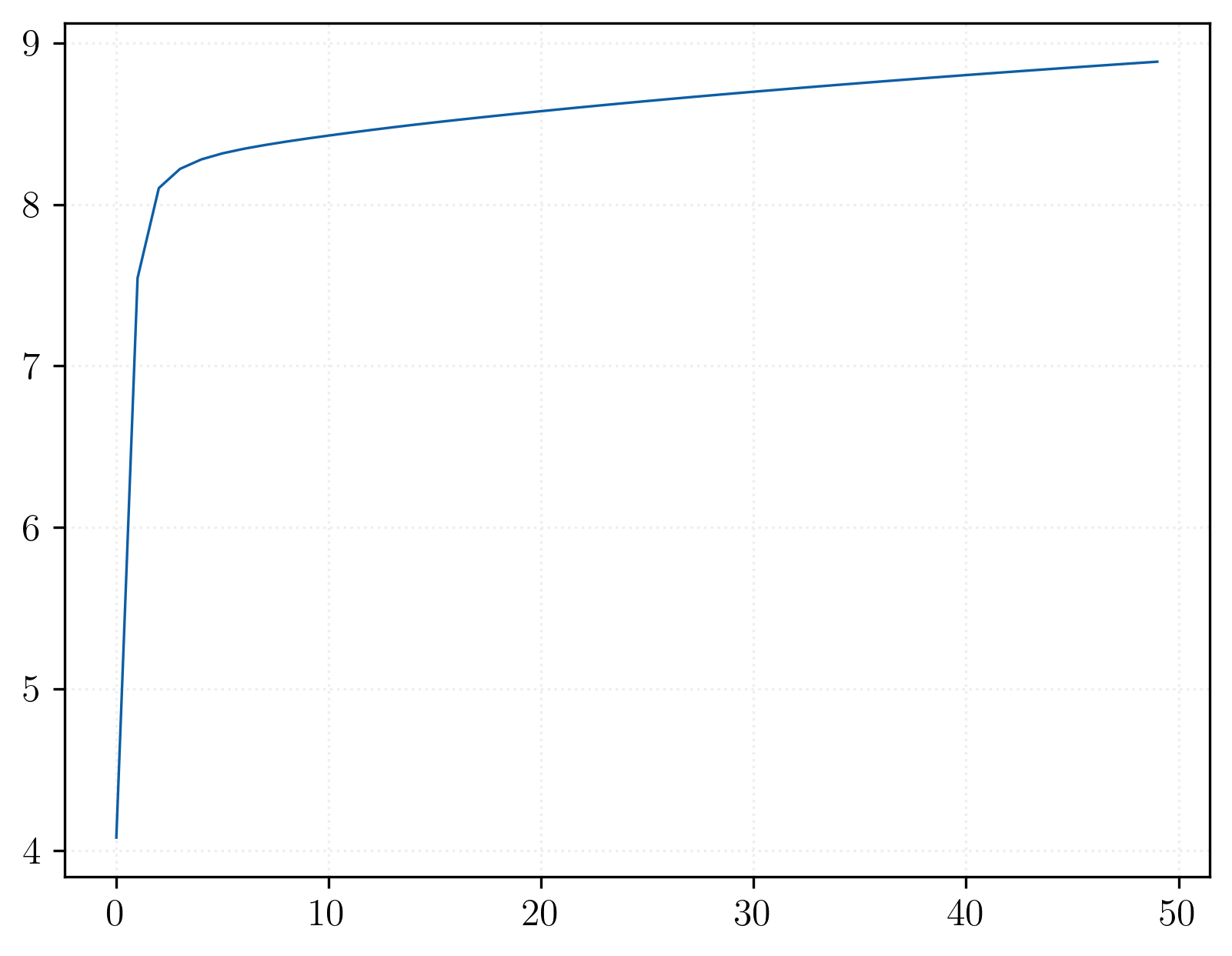
Now we’ll perform the analysis. After each step, use the reactions() method to compute nodal reactions, and retrieve them with nodeReaction.

F = []
for _ in range(50//step):
    analysis.analyze(1)

    # Calculate the reaction forces at the top (y=length)
    model.reactions()
    f = sum(model.nodeReaction(node, 2) for node in find_nodes(model, y=length))

    # Save the reaction force in the list F
    F.append(f)

import matplotlib.pyplot as plt
plt.plot(F)

[<matplotlib.lines.Line2D at 0x30c22afc0>]

Rendering

Now that the analysis is complete, we’ll use the veux library once again to render the displacement and stress fields from the final converged state of the analysis. We’ll draw this in a few stages:

• First create an artist object, which provides detailed control over what will be drawn.

• We’ll begin by invoking draw_outlines which will draw the outlines of the elements in the mesh. Because no arguments are supplied in this first call, the mesh will be drawn in the reference configuration without any deformation.

• Next we’ll invoke draw_outlines again, and this time use the nodeDisp method as the state argument so that the mesh is drawn in the deformed configuration.

from xara.post import NodalStress

artist = veux.create_artist(model)

artist.draw_outlines()
artist.draw_outlines(state=model.nodeDisp, scale=1)
artist.draw_surfaces(state=model.nodeDisp, scale=1, field=NodalStress(model, "syy"))
artist

References

• Abaqus

• Abaqus (Sensitivity)