Moment-Curvature

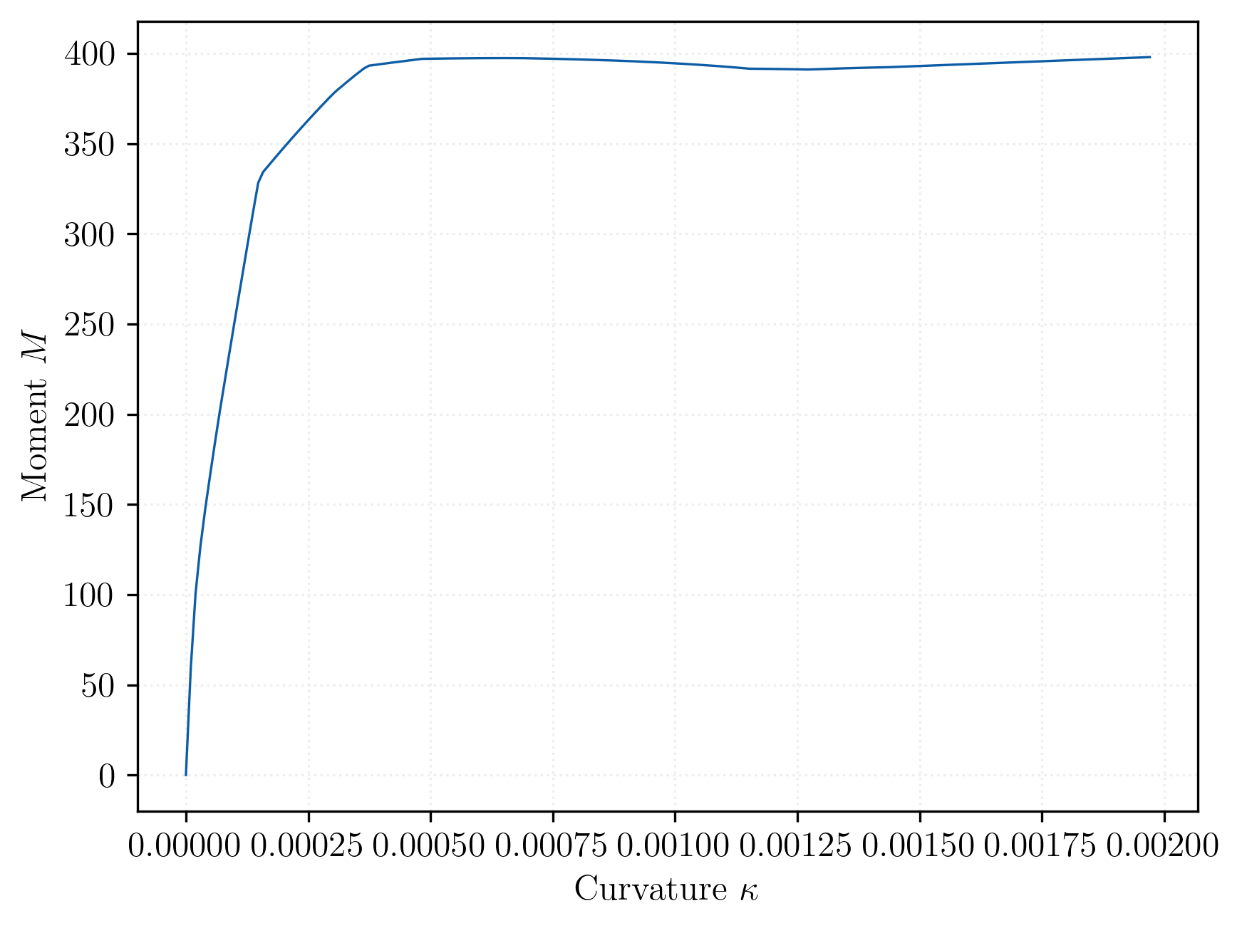
Download notebook

A moment-curvature analysis is performed using a uniaxial fiber section.

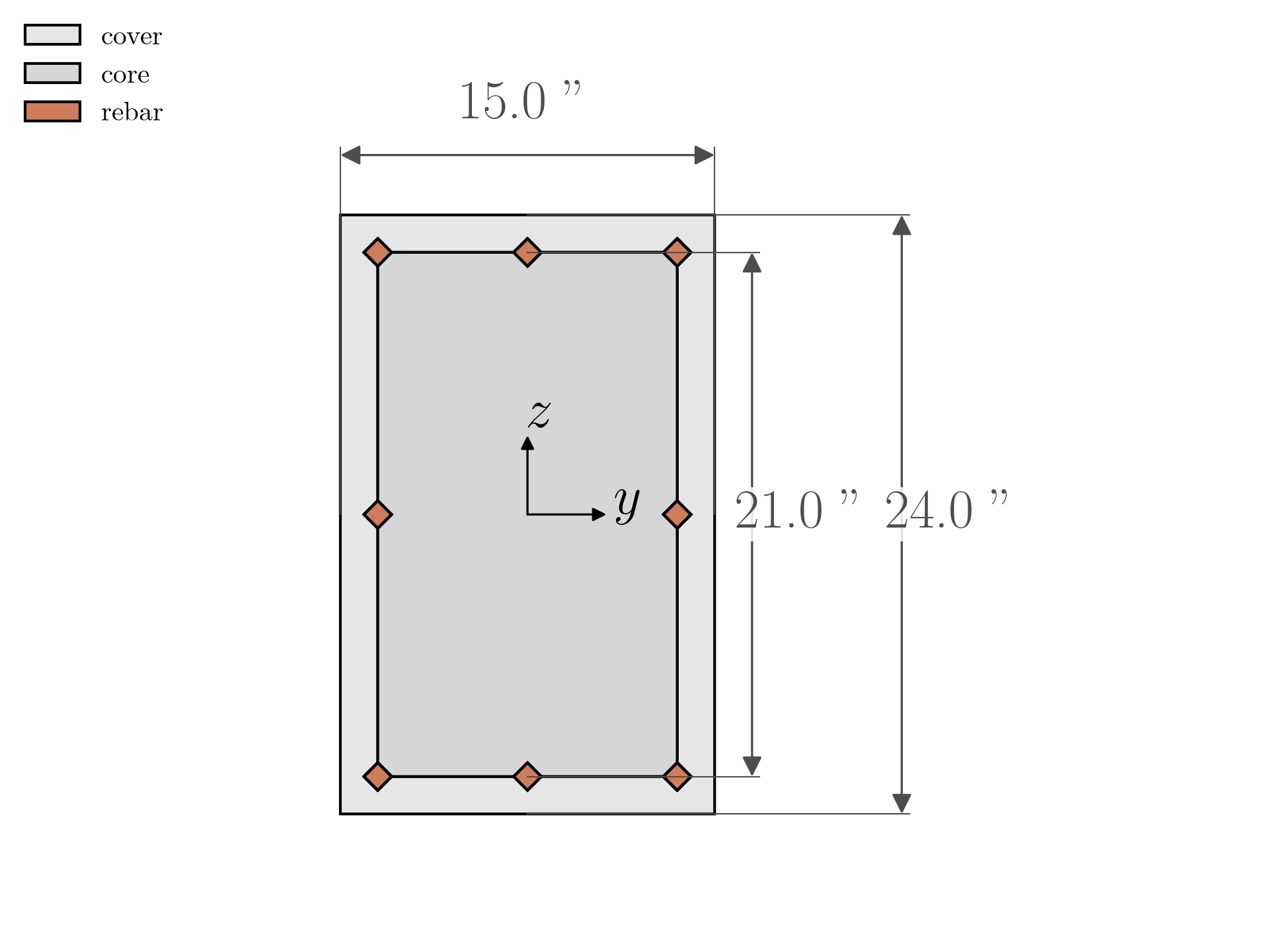
The geometry of the section is depicted below:

Modeling

The primary steps to define the section model are:

1. First we create three instances of xara.UniaxialMaterial to represent the constitutive response.

2. Next a shape is defined which represents the geometry of the section

3. Finally, a xara.FrameSection is created that selects the UniaxialFiber formulation, and specifies the discrete placement of fibers in the section.

Before proceeding, create a helper to keep track of units:

from xara.units import create_units

units = create_units(system="iks")

inch = units.inch 
foot = units.foot
ksi  = units.ksi
kip  = units.kip

Materials

Create three xara.UniaxialMaterials

import xara
Fy = 60*ksi
Es = 29e3*ksi

# Define materials
materials = {
    "core": xara.UniaxialMaterial(
        type = "Concrete01",
        Fc  =  6*ksi,
        nu  =  0.2,
        ec0 =  0.004,
        Fcu =  5*ksi,
        ecu =  0.014
    ),
    "cover": xara.UniaxialMaterial(
        type = "Concrete01",
        Fc  =  -5*ksi,
        nu  =   0.2,
        ec0 =  -0.002,
        Fcu =  -0.0*ksi,
        ecu =  -0.006,
        # "lambda": 0.1,
        # "Ft": 0.65*ksi,
        # "Ets": 500. # Tension stiffening
    ),
    "rebar": xara.UniaxialMaterial(
        type = "Steel01",
        nu = 0.3,
        E  =   29e3*ksi,
        Fy =     60*ksi,
        b =   0.01
    )
}

Section Geometry

The geometry of the section comprises three regions:

• The core of the section is a rectangle

• The cover of the section is a hollow rectangle surrounding the core

• The reinforcement

from xsection import CompositeShape
from xsection.library import Circle, Rectangle, HollowRectangle


# dimensions
b = width = 15.0*inch
h = depth = 24.0*inch
c         =  1.5*inch # cover
r = 0

As = 0.60*inch**2;        # area of no. 7 bars
r_bar = (7/16)*inch;      # radius of rebar

# 1. Core region
core = Rectangle(b-2*c, h-2*c, z=1, 
                 mesh_scale=2,
                 group="core", material=materials["core"])

# 2. Cover region
cover = HollowRectangle(b, h, t=c, z=0, 
                        group="cover", 
                        # mesh_scale=2,
                        material=materials["cover"]
)

# 3. Rebar
bar = Circle(radius=r_bar, 
             z=2, 
             material=materials["rebar"], 
             group="rebar", 
             divisions=4, 
             mesh_scale=1/2)

shape = CompositeShape([
            cover,
            core,
            *bar.linspace([-b/2+c+r, -h/2+c+r], [ b/2-c-r,-h/2+c+r], 3), # Top bars
            *bar.linspace([-b/2+c+r,        0], [ b/2-c-r,       0], 2), # Center bars
            *bar.linspace([-b/2+c+r,  h/2-c-r], [ b/2-c-r, h/2-c-r], 3)  # Bottom bars
        ])

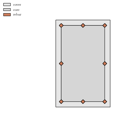
import veux
veux.draw_shape(shape)

Section

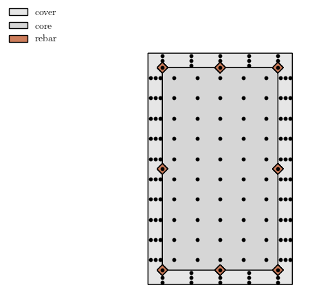
Finally, create the UniaxialFiber section.

fibers = {
    "cover": {"d": 10, "t": 3, "b": 5},
    "core":  {"d": 10, "b": 5},
    "rebar": {"d": 1}
}

section = xara.FrameSection("UniaxialFiber", shape, fibers=fibers)

veux.draw_shape(section)

Model

With the section now defined, we proceed to create a simple xara.Model to perform a moment-curvature analysis. A ZeroLengthSection element is used.

def create_model(section, y=None):
    model = xara.Model(ndm=3, ndf=6)

    # Define two nodes at (0,0)
    model.node(1, (0.0, 0.0, 0))
    model.node(2, (0.0, 0.0, 0))

    # Fix all degrees of freedom except axial and bending
    model.fix(1, (1, 1, 1, 1, 1, 1))
    model.fix(2, (0, 1, 1, 1, 0, 1))

    # Define materials
    for material in materials.values():
        model.material(material)

    # Define section
    model.section(section)

    # Define element
    x = (1.0, 0.0, 0.0)
    if y is None:
        y = (0.0, 1.0, 0.0)

    model.element("ZeroLengthSection", 1, (1, 2), section, y=y, x=x)

    return model

Analysis

The moment curvature analysis proceeds in two phases:

1. First, the axial loading is applied and one analysis step is performed with the analysis_1 object.

2. Next, analysis_2 is created which uses DisplacementControl

import numpy as np

def moment_curvature(section, axialLoad, maxK, numIncr, y=None):
    """
    Arguments
       section -- section to be analyzed
       axialLoad -- axial load applied to section (negative is compression)
       maxK -- maximum curvature reached during analysis
       numIncr -- number of increments used to reach maxK (default 100)
    """
    model = create_model(section, y=y)
    #
    # Apply axial loading
    #

    # Define constant axial load
    model.pattern("Plain", 1, "Constant", 
                  loads={2: [axialLoad, 0.0, 0.0, 0, 0, 0]}
    )

    analysis_1 = xara.StaticAnalysis(model,
        integrator=xara.LoadFactorControl("Proportional", 0.0),
        algorithm="Newton",
        test=xara.Test("NormUnbalance", 1.0e-10, 10)
    )

    # Do one analysis for constant axial load
    analysis_1.analyze(1)

    #
    # Analyze in flexure
    #
    # Define reference moment
    model.pattern("Plain", 2, "Linear")
    model.load(2, (0, 0, 0, 0.0, 1.0, 0.0), pattern=2)

    # Compute curvature increment
    dK = maxK/numIncr


    # Use displacement control at node 2 for section analysis
    analysis_2 = xara.StaticAnalysis(model,
        integrator=xara.LoadFactorControl("DisplacementControl", 2, 5, dK),
        algorithm="Newton",
        test=xara.Test("NormUnbalance", 1.0e-10, 10)
    )

    # Do the section analysis
    M,K = [0], [0]
    for i in range(numIncr):
        status = analysis_2.analyze(1)
        if status != 0:
            print(f"Analysis failed at step {i}")
            break
        else:
            K.append(model.nodeDisp(2, 5))
            M.append(model.getTime())

    return np.array([K,M])

P   =  -180.0   # Axial load
mu  =    15 #32.0   # Target ductility for analysis
numIncr = 200   # Number of analysis increments


# Estimate yield curvature
# (Assuming no axial load and only top and bottom steel)
d = depth - c   # d -- from cover to rebar
epsy = Fy/Es # steel yield strain
Ky = epsy/(0.7*d)
Kz = epsy/(0.7*b)

import matplotlib.pyplot as plt

K, M = moment_curvature(section, P, Ky*mu, numIncr)
plt.plot(K, M/(kip*foot))
plt.grid(True)
plt.xlabel("Curvature $\\kappa$")
plt.ylabel("Moment $M$");