Corotational#
Deprecated since version 0.0.8: This formulation is made obsolete by the new Corotational02 formulation.
Corotational02 corrects several bugs in the original Corotational formulation.
The original Corotational transformation will continue
to be supported to ensure prior investigations remain reproducible, but all new analyses should use the new Corotational02 formulation.
The corotational coordinate transformation performs a geometric transformation from a basic system [1] to the global coordinate system. [2]
- Model.geomTransf("Corotational", tag, vecxz[, offi, offj])
Define a corotational geometric transformation for frame elements.
- Parameters:
- tag: integer
integer tag identifying transformation
- vecxz: tuple of floats
X, Y, and Z components of vecxz, the vector used to define the local x-z plane of the local-coordinate system, required in 3D. The local y-axis is defined by taking the cross product of the vecxz vector and the x-axis.
- offi: tuple of floats
joint offset values – offsets specified with respect to the global coordinate system for element-end node i (optional, the number of arguments depends on the dimensions of the current model).
- offj: tuple of floats
joint offset values – offsets specified with respect to the global coordinate system for element-end node j (optional, the number of arguments depends on the dimensions of the current model).
- geomTransf Corotational $transfTag < $vecxzX $vecxzY $vecxzZ > <-jntOffset $dXi $dYi $dZi $dXj $dYj $dZj>
Argument |
Type |
Description |
|---|---|---|
$transfTag |
integer |
integer tag identifying transformation |
$vecxzX $vecxzY $vecxzZ |
float |
X, Y, and Z components of vecxz, the vector used to define the local x-z plane of the local-coordinate system. The local y-axis is defined by taking the cross product of the vecxz vector and the x-axis. These components are specified in the global-coordinate system X,Y,Z and define a vector that is in a plane parallel to the x-z plane of the local-coordinate system. These items need to be specified for the three-dimensional problem. |
$dXi $dYi $dZi |
float |
joint offset values – offsets specified with respect to the global coordinate system for element-end node i (optional, the number of arguments depends on the dimensions of the current model). |
$dXj $dYj $dZj |
float |
joint offset values – offsets specified with respect to the global coordinate system for element-end node j (optional, the number of arguments depends on the dimensions of the current model). |
Note
The element coordinate system and joint offsets are the same as that documented for the Linear transformation.
Examples#
This example is developed in detail on the examples site. In order to cover a wide range of cases, the strong axis of the first column, element 1, is oriented so as to resist bending outside the plane of the portal, but the strong axis of the second column, element 3, will resist bending inside the portal plane.
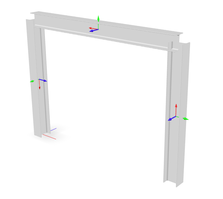
A portal frame with \(X_3\) vertical.#
model.node(1, (    0, 0,      0))
model.node(2, (width, 0,      0))
model.node(3, (width, 0, height))
model.node(4, (    0, 0, height))

model.geomTransf("Corotational", 1, (1, 0, 0)) # Column
model.geomTransf("Corotational", 2, (0, 0, 1)) # Girder
model.geomTransf("Corotational", 3, (0,-1, 0)) # Column
Theory#
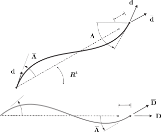
Corotational transformation of a two-node frame.#
The undeformed cross sections of a beam can be represented by a stationary field of three reference directors \(\mathbf{D}_k\) that are orthonormal everywhere in \(\mathcal{B}\). As the beam deforms, these directors are transformed into the deformed directors \(\mathbf{d}_k\)
Under a corotational transformation, an element’s state determination is performed in a transformed configuration space represented by director fields \(\left\{\bar{\mathbf{d}}_k\right\}\), and \(\left\{\bar{\mathbf{D}}_k\right\}\) with the expressions:
Note
It is more appropriate to think of the corotational transformation as a family of transformations.
Figure corot-directors illustrates this for an example embedding where a
single representative director from each of these fields, say
\(k=1\), is shown and \(\mathbf{D}_1\) is taken to be aligned
with the reference configuration of an initially straight plane frame
(note that the subscript 1 will be dropped for clarity). Because
\(\mathbf{D}\) was taken in a straight line for this example and
\(\boldsymbol{R}\) is necessarily homogeneous, it follows from @eq:directors
that \(\bar{\mathbf{d}}\) traces a similar straight line. It is also
useful to observe that @eq:tether implies the following alternative
representation for \(\boldsymbol{R}\), and \(\bar{\boldsymbol{\Lambda}}\) which
is also apparent from the figure above:
where we use the identities \(\left(\boldsymbol{a}\otimes\boldsymbol{b}\right)\left(\boldsymbol{c}\otimes\boldsymbol{d}\right) = \boldsymbol{b}\cdot\boldsymbol{c}\, \left(\boldsymbol{a}\otimes\boldsymbol{d}\right)\) and \((\boldsymbol{a}\otimes\boldsymbol{b})^{\mathrm{t}} = \boldsymbol{b}\otimes\boldsymbol{a}\) and summation is again implied.
If a finite element implements an ideal strain measure that is exactly objective, then such a transformation will by definition be unobservable in the analysis results. However, due to the complexity in the configuration manifold of beams, such a strain measure is almost never used, and consequenty the effect of the corotational transformation is very apparent.
References#
Code Developed by: Remo Magalhaes de Souza, Claudio M. Perez